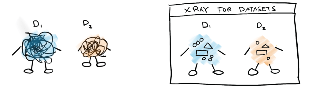
Where’s the theory on datasets?

The canonical model of splitting a dataset into train and test data allows statistical validity for the evaluation of model performance. However, in the real world, there is often not only one source of data to consider but many different sources; the construction and processing of the training set is far from straightforward. On one hand, bespoke data for a specific application may be very limited or not available at all. On the other hand, using all possible data sources may also cause a plethora of issues including distributional mismatch and reduced data quality. Given that the quality, size, and composition of different data sources may vary; it is currently unclear how data curation affects downstream model performance.

A recent line of empirical work has investigated and optimized data composition for various types of models and downstream tasks. However, there is limited work in modeling and analyzing the theoretical properties of different scenarios of data composition. Data curation is a difficult problem due to the large search space for optimal data composition. Prior works thus far have seldom formalized theoretical models for this generalized data composition problem. Existing works have studied models for describing mixtures of data in language modeling [XPD+23] and the role of noise in scaling laws [BDK+21] . This blog post focuses on the specific empirical scenario of removing data points within a training set. We will examine the different theoretical models proposed for this setting.

Four Theoretical Models of Data Deletion

Our scope is theoretical models which study the effect of the removal of a subset of training data. Let be the original dataset and let be a smaller dataset that is a subset of . Let represent the parameters for some model of interest.

View 1: Influence Perturbations and the Estimating Effect Size

In An Automatic Finite-Sample Robustness Metric: When can dripping a Little Data Make a Big Difference [BGM20], we draw our first view of removing data to approximate the influence of different points in the training set. Influence functions have been widely used in various machine-learning settings as linear approximations for the effect of training data on a specific test instance [Law86, KL17].

Motivated by the sensitivity of applied econometric studies to small changes in the study samples, Broderick, Giordano, and Meager model how the composition of survey data can drastically affect the conclusions of different studies. In particular, they introduce a metric Approximate Maximum Influence Perturbation; a measure of the sensitivity of conclusions to the removal of a small fraction of the sample data. If a small fraction of data can significantly change the effect direction or the significance of an effect, then the conclusions based on the observed effect may be cast into doubt.

To test the impact of removing a small sample on the quantity of interest, the Maximum Influence Perturbation is the largest possible change induced in the quality of interest by dropping no more than of the dataset and The Most Influential Set is then the set that achieves the Maximum Influence Perturbation .

More formally, let be the weights of a dataset of size where . Let be the parameters of a linear model and be the quantity of interest (e.g. effect size). Let be the estimator for a specific set of weights () and is the quantity of interest when all the examples are included, then the Most Influential Set can be identified using the weights :

Since it is difficult to find these weights exactly without refitting a model for every possible , the work mainly focuses on the Approximate Maximum Influence Perturbation, , as an approximation for the largest possible change induced in the quality of interested by dropping no more than fraction of data. For this approximation, they use the first-order Taylor expansion of at :

.

Thus the Approximate Maximum Influence Perturbation (AIMP) is then:

Practically, finding this perturbation involves first fitting a model on all of the data points to find and then computing the approximate value of for each and then selecting the most negative values to remove to induce the largest change.

Empirical Findings: The authors use this analysis to check the AMIP robustness for several empirical studies including the Oregon Medicaid RCT [FTW+12] and the Progresa Cash Transfers RCT [ADG09] to find that the estimated treatment effects can be reversed by dropping less than 1% of the sample.

Similar to prior work, this work also assumes the linear composition of data point influence when approximating the overall effect of removing a group of points. Since the scope of the models studied is limited to OLS-fitted linear models, their linear assumptions give good approximations to the true behavior of removing data.

View 2: Extreme Value Theory and Subgroup Performance

In the next approach, we move on to thinking about deleting data for maximum margin SVMs in Why Does Throwing Away Data Improve Worst-Group Error [CAALP23]. Canonical learning theory results show that adding more data should improve generalization error. However, when there are subgroups in the dataset, prior empirical results have found that throwing away samples until classes are balanced is better for the worst group than using all the data points [IAPLP22]. This work focuses on the setting of linear maximum-margin binary classifiers and examines how decision boundaries are changed or improved by balancing data by leveraging results from extreme value theory.

Let be the features vectors, be the labels, be the binary sensitive attributes, and $w$ once again be the weights. The maximum margin classifiers (SVMs) for classes A, B defined by find the following optimal parameters:

It is important to note that groups are defined over both sensitive attributes and labels (i.e. ). Describing the behavior of and based on the tail properties of the data distribution will be the strategy for characterizing the worst group performance. The paper describes two types of distributions: the Weibell family and the Gumbel family. For example, the Gumbel-type distributions have small tails such as Gaussian and Exponential while Weibull distributions include the Uniform distribution. The Fisher-Tippet-Gnedenko theorem characterizes the maximum value and tail behaviors from these two families of distributions. Using these descriptions, if training data in the majority class is more spread out, it would bias the ERM output and result in a lower worst-group accuracy.

	Gumbel Distributions	Weibull Distributions
Worst-class error	ERM error ≥ Subsampling Error	ERM error ≤ Subsampling Error
Worst-group error	ERM error ≥ Subsampling Error	ERM error ≤ Subsampling Error

The implications are summarized in the table above which describes the errors with constant probability for linearly separable data for the low dimensional case. Using the properties of each family of distributions, they give a lower bound for and upper bound for for general Gumbel distributions and vise-versa for Weibull-type distributions. From there under linearly separable conditions, we can discern the relationship between worst class error using empirical risk minimization and subsampling. For worst group error, defined over both sensitive attributions and labels, Weibull-type distributions converge to the optimal worst group error classifier under ERM.

Empirical Findings: Using two image datasets, Waterbirds and CelebA, the authors find that sub-sampling outperforms empirical risk minimization applied directly. Because the theoretical results are based on low-dimensional settings, the researchers tested these classification problems by fitting predictors to the top few features. They also study the distribution of top principal components of these features and found long-tailed behavior that is closer to the Gumbel family where the theoretical results indeed suggest that the worst group would experience lower error through subsampling.

This work frames data deletion as balanced subsampling, wherein data from the majority groups and classes are selected for deletion. There is a binary choice here in either using the full sample or using the balanced subsample rather than the deletion of individual points in the dataset. This work also differs from the other works discussed here in that it focuses on the effects of removing data on the worst subgroup in particular. Furthermore, in the context of machine learning, the primary concern shifts from focusing on a specific parameter of interest to minimizing error.

View 3: Gradient Tracing for Data Pruning

Moving on to the deep learning setting, we examine works that investigate data pruning to improve training efficiency. This work, Deep Learning on a Data Diet: Finding Important Examples Early in Training [PGD21], proposes strategies for optimal data deletion by examining the training gradients.

The default practice in deep learning is to include the entire training dataset for training the model. However, it is not clear if all data points are necessary, particularly for noisy datasets or datasets with a lot of repetition. Ideally, developing a heuristic to identify which samples to prune would help identify which examples to include and exclude. In this paper, the authors propose two score functions to approximately measure the change in loss from removing a sample and use these scores to prune the training dataset.

Let be a dataset, where , , and are the parameters of the neural network. The loss is calculated using cross-entropy loss , where represents the probabilities of each class given a set of weights. Let be the gradient of a training example at time $t$. The gradient norm score (GraNd) is:

.

This measure is proposed as an approximation of the gradient contribution of a specific example at time . However, in the case where the gradient of the weights with respect to the logits is similar across logits and training examples, the gradient norm score can be further approximated by the norm of the error vector. Thus the error L2-Norm score is:

.

Empirical Findings: In their empirical results, the authors find that the EL2N score becomes an accurate approximation after a few epochs of training. When pruning according to the EL2N score, they found that removing 60% of CIFAR10 and 30% of CIFAR100 still yielded the same test accuracy. Since a random pruning strategy resulted in much worse accuracy, this suggests that not all examples are equally important in the training of these large models. Furthermore, they find that computing the EL2N score in the 4-8th epoch is sufficient to find an effective pruning strategy. The paper also finds that if only 10% of examples could be included for training, test accuracy increases with the inclusion of more difficult examples, reaching its peak at the most difficult decile of examples.

While in the previous two works, the focus was on understanding the change removing data produces, this work asks how performance might stay the same with data removed. Rather than evaluating importance through the influence functions, this work considers gradients of training examples. In fact, if influence functions are measured in the final model, E2LN score can be estimated near the beginning of training.

View 4: Gardner’s Theory for Beating Neural Scaling Laws

The next work is a different perspective on data composition, instead of asking about pruning, this work asks whether data can be strategically selected to improve on the empirical phenomenon of power-law scaling. This work shares the same objective of View 3 in improving the efficiency of model training but adds an underlying model inspired by statistical mechanics. Motivated by existing examples of power scaling laws with small exponentials, the paper Beyond neural scaling laws: beating power law scaling via data pruning [SGS+22] asks whether power-law scaling can be improved by selecting data strategically.

In this model, they assume that there is a training set where . They also defined a student perceptron weight vector and a teacher perceptron weight vector with the dataset labels coming from . And is the ratio between the number of training samples and the dimension of the parameters (i.e. ).

To select training data, the student probe model is trained for a few epochs, and then margins can be calculated for each example with respect to (i.e. ). Then a training dataset can be constructed with a specified fraction of examples. The goal of the theoretical model presented in this work is to estimate the error using , fraction of examples kept , and the distance between the student probe and teacher (i.e. . Using these three inputs, the governing equations provided by a statistical mechanics model: the replica model using Gardner’s volume that can then be used to estimate the error of the full student model. At a high level, these equations are derived by computing the volume of solutions that perfectly classify training data up to some margin.

Empirical Findings: In their empirical experiments, they find that the best pruning strategy actually depends on the amount of initial data. If is large, keeping the hardest examples performs better, and if is small, keeping the easier examples performs better. They demonstrate these results on popular image classification benchmarks such as CIFAR10 and ImageNet. They also present experiments measuring information gain (the change in entropy over the student perceptron weights), and find that as data pruning is more aggressive the information gain per new sample increases. In the limit, information gain goes to 0 in the power law case with no pruning and infinite samples.

This paper not only uses a heuristic to prune examples but also explains the behavior of pruning with an underlying model from replica theory. While their empirical simulations do match their theoretical curves, it is unclear whether this theory is the only way to explain why pruning examples improve the data efficiency of training. The interesting takeaway from their theory is that the decision to keep difficult or easy examples depends on the amount of initial data available. This extends the observations of previous work, indicating that keeping the most difficult examples is not desirable when using only 10% of the training data.

Summary

These four works present unique theoretical models explaining the impact of removing examples from training datasets. They collectively demonstrate that efficiency and fairness can be improved by strategic data point removal. This insight opens up several intriguing avenues for future research:

1. Data Selection: Developing algorithms to optimize not just overall performance, but also robustness and fairness.
2. Optimization Dynamics: Modeling how data ordering and composition affect training dynamics and model optimization.
3. Dataset Quality Metrics: Creating measures to assess dataset quality, especially for pre-training datasets across various domains.
4. Quality-Aware Scaling Laws: Integrating data quality considerations into scaling laws to better predict efficiency, accuracy, and reliability of future models.

In the era of foundation models, finding theoretically grounded methods for efficient data selection is a promising approach to mitigate the growing environmental impact of AI research.

Acknowledgements

This blog post is a part of my theory qualifiying exams. Special thanks to Omer Reingold, John Duchi, and Greg Valiant for being on my quals committee and Mansheej Paul for feedback on this post.

References

[ADG09] Manuela Angelucci and Giacomo De Giorgi. Indirect effects of an aid program: how do cash transfers affect ineligibles’ consumption? American economic review, 99(1):486–508, 2009.
[BDK+21] Yasaman Bahri, Ethan Dyer, Jared Kaplan, Jaehoon Lee, and Utkarsh Sharma. Explaining neural scaling laws. arXiv preprint arXiv:2102.06701, 2021.
[BGM20] Tamara Broderick, Ryan Giordano, and Rachael Meager. An automatic finite-sample robustness metric: when can dropping a little data make a big difference? arXiv preprint arXiv:2011.14999, 2020.
[CAALP23] Kamalika Chaudhuri, Kartik Ahuja, Martin Arjovsky, and David Lopez-Paz. Why does throwing away data improve worst-group error? In International Conference on Machine Learning, pages 4144–4188. PMLR, 2023.[FTW+12] Amy Finkelstein, Sarah Taubman, Bill Wright, Mira Bernstein, Jonathan Gruber, Joseph P Newhouse, Heidi Allen, Katherine Baicker, and the Oregon Health Study Group. The oregon health insurance experiment: evidence from the first year. The Quarterly journal of economics, 127(3):1057–1106, 2012.
[IAPLP22] Badr Youbi Idrissi, Martin Arjovsky, Mohammad Pezeshki, and David Lopez-Paz. Simple data balancing achieves competitive worst-group-accuracy. In Conference on Causal Learning and Reasoning, pages 336–351. PMLR, 2022.
[KL17] Pang Wei Koh and Percy Liang. Understanding black-box predictions via influence functions. In International conference on machine learning, pages 1885–1894. PMLR, 2017.
[Law86] John Law. Robust statistics—the approach based on influence functions, 1986.
[PGD21] Mansheej Paul, Surya Ganguli, and Gintare Karolina Dziugaite. Deep learning on a data diet: Finding important examples early in training. Advances in Neural Information Processing Systems, 34:20596–20607, 2021.
[SGS+22] Ben Sorscher, Robert Geirhos, Shashank Shekhar, Surya Ganguli, and Ari Morcos. Beyond neural scaling laws: beating power law scaling via data pruning. Advances in Neural Information Processing Systems, 35:19523–19536, 2022.
[XPD+23] Sang Michael Xie, Hieu Pham, Xuanyi Dong, Nan Du, Hanxiao Liu, Yifeng Lu, Percy Liang, Quoc V Le, Tengyu Ma, and Adams Wei Yu. Doremi: Optimizing data mixtures speeds up language model pretraining. arXiv preprint arXiv:2305.10429, 2023.