Suppose that is an unknown binary string of length . We are asked to recover from its traces, and each trace is a random subsequence obtained by deleting the bits of independently with probability .
More formally, let denote the distribution of traces obtained from string . For example, when , assigns a probability mass of to each element in the multiset
We then ask: what is the smallest number such that we can recover any (say, with probability ) given independent samples from ?
This trace reconstruction problem was first formulated by Batu-Kannan-Khanna-McGregor in 2004, and their central motivation is from the multiple sequence alignment problem in computational biology. Trace reconstruction is also a fundamental problem related to the deletion channel in communication theory: We view the hidden string as the transmitted message, and each trace as a received message that went through a deletion channel, which drops each bit with probability . Then the sample complexity tells us the number of independent copies that need to be sent for the receiver to determine the original message.
Despite being a natural problem, trace reconstruction is still far from being well-understood, even from the information-theoretic perspective (i.e., without considering the computational complexity). In 2017, De-O’Donnell-Servedio and Nazarov-Peres independently proved . A very recent breakthrough due to Chase further improved this bound to , which is still super-polynomial. On the other hand, the best known sample complexity lower bound is merely , proved by Chase in another recent work.
In this blog post, I will explain why this problem is much more non-trivial than it might appear at first glance. I will also give an overview on the work of [DOS17, NP17], which, interestingly, reduces this seemingly combinatorial problem to complex analysis.
Observation: reconstruction distinguishing TV-distance. Let us start with a natural first attempt at the problem. Define as the minimum statistical distance between the trace distribution of two different length- strings:
It is not hard to show that bounds on both sides, up to a polynomial factor:
The lower bound holds because any trace reconstruction algorithm must be able to distinguish from for every pair of different strings , and this requires samples for the minimizer in the definition of . For the upper bound, we note that every pair can be distinguished with an error probability using samples. We say that string “beats” , if the distinguisher for decides that ““. By a union bound, the correct answer “beats” every other string with high probability. We can then obtain a reconstruction algorithm by running the distinguisher for every string pair, and outputting the unique string that “beats” the other strings.
Thus, to determine whether the sample complexity is polynomial in , it suffices to determine whether scales as or is much smaller. Unfortunately, it turns out to be highly non-trivial to bound , and even bounding for “simple” and can be hard. Imagine that we try to reason about the distribution : the probability mass that assigns to string is proportional to the number of times that appears as a subsequence in , but this count is already hard to express or control, unless has a very simple pattern. This is roughly where this natural attempt gets stuck.
Distinguishing using estimators. Now we turn to a different approach that underlies the recent breakthrough on trace reconstruction algorithms. As discussed earlier, we can focus on the problem of distinguishing the case from for fixed strings . Let be a function defined over all possible traces from a length- string. We consider the following algorithm for distinguishing from :
Step 1. Given traces , compute the average of Step 2. Output if the average is closer to than to , and output otherwise.
For the above to succeed, needs to satisfy the following two conditions:
(Separation) and are well-separated under , namely for some . (Boundedness) Expectation of can be efficiently estimated. This can be guaranteed if for some , holds for every .
Assuming the above, a standard concentration argument shows that we can distinguish and using samples, and thus .
In principle, a near-optimal choice of would be setting to be the indicator of , which gives boundedness and separation . However, as argued above, this optimal choice of can still be hard to analyze. Instead, we focus on choosing a simpler function , which potentially gives a suboptimal but admits simple analyses.
Sketch of the Upper Bound. The main results of [DOS17] and [NP17] follow from choosing to be a linear function. Given a trace , we consider the following polynomial with coefficients being the bits of :
For some number to be determined later, we consider the estimator , which is indeed a linear function in the trace .
At first glance, it might be unclear why we choose the coefficients to be powers of . The following fact justifies this choice by showing that polynomials interact with the deletion channel very nicely: The expectation of is exactly the evaluation of the polynomial with coefficients , but at a slightly different point.
Fact: For any string ,
Equivalently, we have , which allows us to rephrase our requirements on the choice of as follows:
(Separation) for some that is not too small. (Boundedness) for all possible trace , for some that is not too large.
After some thought, it is beneficial to choose such that both and are close to , since this ensures that different bits in the string are assigned weights of similar magnitudes in the polynomials above. These two conditions hold if and only if .
The overall plan for distinguishing strings and .
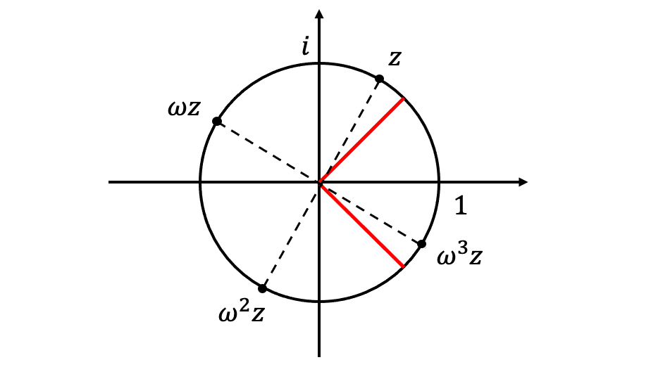
The crucial idea in both papers [DOS17, NP17] is to consider the polynomials in the complex plane instead of on the real line. Fortunately, all the previous discussion still holds for complex numbers, with interpreted as modulus instead of absolute value. In [NP17], the authors chose from a small arc of the unit circle:
.
Arc marked by the red box and dotted lines.
For every , it is easy to upper bound : it follows from simple calculus that , and thus for every :
.
To lower bound , note that since both and are binary, all the coefficients of are in . Such polynomials are known as Littlewood polynomials. The separation condition is then reduced to the following claim in complex analysis:
Littlewood polynomials cannot to be too “flat” over a short arc around 1.
By Lemma 1, there exists such that the separation condition holds for . Recall that the boundedness holds for . This shows that the sample complexity is upper bounded by , which is minimized at . This proves the upper bound .
Proof of a weaker lemma. While the original proof of Lemma 1 is a bit technical, [NP17] presented a beautiful and much simpler proof of the following weaker result, in which the lower bound is replaced by , where is the degree of the Littlewood polynomial.
Lemma 2. ([Lemma 3.1, NP17]) For every nonzero Littlewood polynomial of degree ,
.
Proof. Without loss of generality, we assume that the constant term of is . Suppose otherwise, that the lowest order term of is for some . We may consider the polynomial instead.
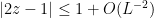
Let be the maximum modulus of over arc , and be an -th root of unity. Consider the following polynomial:
.
For every on the unit circle, at least one point falls into the arc , so that . (See figure below for a proof by picture.) The moduli of the remaining factors are trivially bounded by . Thus, .
On the other hand, we note . The maximum modulus principle implies that for some on the unit circle, we have . Therefore, we must have , which implies and completes the proof.
Points involved in the definition of for . In this case, is inside arc , which is marked by the red lines.
Beyond linear estimators? The work of [DOS17, NP17] not only proved the upper bound, but also showed that this is the best sample complexity we can get from linear estimator . The recent work of [Cha20] goes beyond these linear estimators by taking the higher moments of the trace into account. The idea turns out to be a natural one: consider the “-grams” (i.e., length- substrings) of the string for some . In more detail, we fix some string , and consider the binary polynomial with coefficients corresponding to the positions at which appears as a (contiguous) substring. The key observation is that there exists a choice of such that the resulting polynomial is sparse (in the sense that the degrees of the nonzero monomials are far away). The technical part of [Cha20] is then devoted to proving an analogue of Lemma 1 that is specialized to these “sparse” Littlewood polynomials.
Acknowledgments. I would like to thank Moses Charikar, Li-Yang Tan and Gregory Valiant for being on my quals committee and for helpful discussions about this problem.
This is an excellent overview of the topic. It makes the connection between complex analysis and the trace reconstruction problem obvious, which is just what I was hoping for.


![\mathbb{E}_{\tilde x \sim \mathcal{D}_x}[f(\tilde x)]](https://s0.wp.com/latex.php?latex=%5Cmathbb%7BE%7D_%7B%5Ctilde+x+%5Csim+%5Cmathcal%7BD%7D_x%7D%5Bf%28%5Ctilde+x%29%5D&bg=ffffff&fg=000000&s=0&c=20201002)
![\mathbb{E}_{\tilde y \sim \mathcal{D}_y}[f(\tilde y)]](https://s0.wp.com/latex.php?latex=%5Cmathbb%7BE%7D_%7B%5Ctilde+y+%5Csim+%5Cmathcal%7BD%7D_y%7D%5Bf%28%5Ctilde+y%29%5D&bg=ffffff&fg=000000&s=0&c=20201002)


![|\mathbb{E}[f(\tilde x)] - \mathbb{E}[f(\tilde y)]| \ge \epsilon](https://s0.wp.com/latex.php?latex=%7C%5Cmathbb%7BE%7D%5Bf%28%5Ctilde+x%29%5D+-+%5Cmathbb%7BE%7D%5Bf%28%5Ctilde+y%29%5D%7C+%5Cge+%5Cepsilon&bg=ffffff&fg=000000&s=0&c=20201002)


![\mathbb{E}_{\tilde s \sim \mathcal{D}_s}\left[\tilde S(z)\right] = \frac{1}{2}S\left(\frac{z+1}{2}\right).](https://s0.wp.com/latex.php?latex=%5Cmathbb%7BE%7D_%7B%5Ctilde+s+%5Csim+%5Cmathcal%7BD%7D_s%7D%5Cleft%5B%5Ctilde+S%28z%29%5Cright%5D+%3D+%5Cfrac%7B1%7D%7B2%7DS%5Cleft%28%5Cfrac%7Bz%2B1%7D%7B2%7D%5Cright%29.&bg=ffffff&fg=000000&s=0&c=20201002)
![\mathbb{E}[\tilde S(2z-1)] = \frac{1}{2}S(z)](https://s0.wp.com/latex.php?latex=%5Cmathbb%7BE%7D%5B%5Ctilde+S%282z-1%29%5D+%3D+%5Cfrac%7B1%7D%7B2%7DS%28z%29&bg=ffffff&fg=000000&s=0&c=20201002)


![A_L = \{e^{i\theta}: \theta\in[-\pi/L, \pi/L]\}](https://s0.wp.com/latex.php?latex=A_L+%3D+%5C%7Be%5E%7Bi%5Ctheta%7D%3A+%5Ctheta%5Cin%5B-%5Cpi%2FL%2C+%5Cpi%2FL%5D%5C%7D&bg=ffffff&fg=000000&s=0&c=20201002)
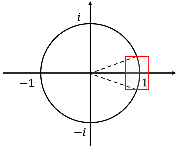
 marked by the red box and dotted lines.

![\left|\tilde S(2z-1)\right| \le \sum_{k=0}^{n-1}\left|(2z-1)^k\right| \le n \cdot \left[1 + O(L^{-2})\right]^n = e^{O(n/L^2)}](https://s0.wp.com/latex.php?latex=%5Cleft%7C%5Ctilde+S%282z-1%29%5Cright%7C+%5Cle+%5Csum_%7Bk%3D0%7D%5E%7Bn-1%7D%5Cleft%7C%282z-1%29%5Ek%5Cright%7C+%5Cle+n+%5Ccdot+%5Cleft%5B1+%2B+O%28L%5E%7B-2%7D%29%5Cright%5D%5En+%3D+e%5E%7BO%28n%2FL%5E2%29%7D&bg=ffffff&fg=000000&s=0&c=20201002)


![q(0) = [p(0)]^L = 1](https://s0.wp.com/latex.php?latex=q%280%29+%3D+%5Bp%280%29%5D%5EL+%3D+1&bg=ffffff&fg=000000&s=0&c=20201002)


 for
for  .
. is inside arc


This is an excellent overview of the topic. It makes the connection between complex analysis and the trace reconstruction problem obvious, which is just what I was hoping for.
LikeLike