By Steve Mussmann and Jacob Steinhardt.
The celebrated pigeonhole principle says that if we have disjoint sets ![S_1, S_2, \dots, S_m \subseteq [n]](https://s0.wp.com/latex.php?latex=S_1%2C+S_2%2C+%5Cdots%2C+S_m+%5Csubseteq+%5Bn%5D&bg=ffffff&fg=000000&s=0&c=20201002) each of size
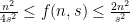
each of size  , then
  (the number of sets) is at most
  .
.
Suppose that instead of being disjoint, we require that every pair of sets has intersection at most  . How much can this change the maximum number of sets ? Is it still roughly
  , or could the number be much larger? Interestingly, it turns out that there is a sharp phase transition at
  ; this is actually the key fact driving the second author’s recent paper on planted clique lower bounds (see the end of this post for some more details on this). These set systems are known as “combinatorial designs” and are heavily studied.
The phase transition is as follows: if  , then
  (as is the case with disjoint sets), while if
  then
then  . Remarkably, even though there can be at most
  sets of size , it is possible to have as many as
  sets of size
  (if
(if  for prime
  ).
).
To be a bit more formal, let  be the maximum number of subsets of
 ![[n]](https://s0.wp.com/latex.php?latex=%5Bn%5D&bg=ffffff&fg=000000&s=0&c=20201002) of size with pairwise intersection sizes at most (i.e.,
of size with pairwise intersection sizes at most (i.e.,  and
and  for
for  ). Assume that
  and
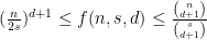
and  . Then,
 for , and
 for .
for .
Below we will show how to give upper and lower bounds on in the case where . (The case is a relatively straightforward application of inclusion-exclusion together with pigeonhole.)
Upper bound
Suppose we have sets ![S_1, ..., S_m \subseteq [n]](https://s0.wp.com/latex.php?latex=S_1%2C+...%2C+S_m+%5Csubseteq+%5Bn%5D&bg=ffffff&fg=000000&s=0&c=20201002) . For each
. For each ![j \in [n]](https://s0.wp.com/latex.php?latex=j+%5Cin+%5Bn%5D&bg=ffffff&fg=000000&s=0&c=20201002) , we will define
, we will define  to be all the sets
  that contain
  . Namely,
  . Note that all sets in have a pairwise intersection at the element and thus must be non-intersecting in
 ![[n] \backslash \{j\}](https://s0.wp.com/latex.php?latex=%5Bn%5D+%5Cbackslash+%5C%7Bj%5C%7D&bg=ffffff&fg=000000&s=0&c=20201002) . Thus, by pigeonhole,
. Thus, by pigeonhole,  . Further, note that each occurs in
  distinct sets . Putting these together, we thus have
 .
.
This yields  , and hence
  .
.
Lower Bound

Intuitively, organize into a rectangle with rows and  columns (put any remaining elements off to the side). See figure above. Note that all columns of the rectangles are sets of size without any intersections and constitute
  sets. Further, we can add the sets composed of the diagonals and anti-diagonals (wrapping around on the left and right sides of the rectangle) which are sets of size without any pairwise intersections of size more than one. This will get us to
  sets. We could attempt to create sets from more “generalized diagonals” where we start at the top of the rectangle and go horizontally by
  columns for every row that we go down (and wrap around on the left and right sides). However, if is divisible by , these “generalized diagonals” would intersect some columns in two places instead of one.
However, if is prime, then all such “generalized diagonals” will intersect each other in at most one point. More precisely, for every  , we can create a set by taking the elements of the rectangle
  for every row
  . There will be
  such sets that will all have size and will have pairwise intersections of size at most one since linear functions have at most one intersection over finite fields.
By Bertrand’s Postulate and since , there is some prime number such that  . We can use this as number of columns in a rectangle. Note that we need
  which is satisfied since . The number of “generalized diagonals” is as mentioned above. Thus, we have explicitly constructed sets of size with pairwise intersections at most one where

and hence  as claimed.
Generalization to Larger Intersections
In general, what if we allow the sets to have intersections of size  ? The above sections study the case where
  , but the basic arguments generalize to larger values of as well. In particular, we have
 for ,
for ,
 for
for 
where  is the maximum number of possible subsets of of size with pairwise intersections at most . Note that this leaves open the question of what happens for
  ; in fact, there appears to be a phase transition around
  , but that is beyond the scope of this post.
Relationship to Planted Clique
The fact that there can be a large number of sets with small intersection when is actually a large part of the motivation behind this recent paper on a lower bound for the semi-random planted clique problem. To quote from the abstract, in the semi-random model, first “a set  of vertices is chosen and all edges in are included; then, edges between and the rest of the graph are included with probability
  , while edges not touching are allowed to vary arbitrarily.”
Clearly, if the clique has size then it is possible to create identical cliques (since we can choose the edges between the remaining  vertices arbitrarily). To handle this ambiguity, we also specify one vertex
  which is guaranteed to be in the planted clique . If
 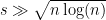 then this is enough to uniquely identify the planted clique with high probability.
However, if  , then it is possible to create
  cliques such that every vertex lies in exactly two cliques, and all cliques intersect in at most element. Moreover, if we choose the cliques appropriately then it is information-theoretically difficult to tell which of the cliques was the original planted clique . As a result, no matter which vertex is specified, we cannot recover with probability greater than (since we can’t distinguish from the other clique that belongs to).
Here, having an intersection size of (rather than a much larger intersection) is key, because this makes it possible to “steal” from the random edges between and ![[n] \backslash S](https://s0.wp.com/latex.php?latex=%5Bn%5D+%5Cbackslash+S&bg=ffffff&fg=000000&s=0&c=20201002) to create additional cliques that intersect with . If the intersection size was instead
to create additional cliques that intersect with . If the intersection size was instead  , then with high probability there would be no subset of vertices of that had a common neighbor outside of , and so there would be no way to create a clique
  that intersected in elements.

That’s pretty cool! I wonder if this can be used to explain some statistical mechanics effects or condensed matter effects, since there’s an approach to stat mech using combinatorics.
LikeLike
Such set families have been studied in the literature on packings, designs, and cover-free families, eg Erdos-Frankl-Furedi 85 and Rodl 85. See Lemma 13 and Prop 14 in http://people.seas.harvard.edu/~salil/research/trev-abs.html for pointers.
LikeLike
Sorry, I see now that you are aware of the literature on designs. I didn’t have a chance to think about the parameter range that you’re interested in, but explicit constructions for some parameter ranges are discussed in Nisan-Wigderson and in Buhrman-Miltersen-Radhakrishnan-Ta-Shma and perhaps other places in the TCS literature.
LikeLike
.. last reference should be Buhrman-Miltersen-Radhakrishnan-Venkatesh
LikeLike
Thanks! If I understand the Nisan-Widgerson construction, I believe that in the language of this post it says that there are subsets of {1, …., n} such that:
(1) Each set has size s = sqrt(n)
(2) Every pair of sets has intersection at most d
(3) The number of sets is 2^d
This shows that if we allow d to grow at a rate faster than log(n), the number of sets actually grows superpolynomially. Actually I believe that this is true even if d = omega(1), based on the “Generalization to Larger Intersections” given in the post.
LikeLike
Great post! There are a couple of points that confused me (which are clarified on reading the paper):
1) The edges in ~S are chosen after the random edges between S and ~S.
2) v is sampled randomly from S, after the graph is fixed. (If it is chosen along with S before fixing the other edges, it’s easy to make multiple cliques that intersect only on v).
LikeLike
Yes, thanks! Both of your clarifications are correct.
LikeLike
Nice post!! out of a universe of size
  then the expected size of the intersection is
  .
.
More generally, if you choose random sets of size
Once you allow the intersection size to be about that size, then you can have combinatorial designs with exponentially more sets than otherwise.
This is also the key insight behind the Nisam-Wigserson pseudorandom generator (where one sets the intersection size to be roughly logarithmic in the size of circuit one is trying to fool).
LikeLike
Yes, the value for random sets seems to be the key threshold; however from this it wasn’t obvious to me how to get the right order of growth in the number of sets once we pass that threshold. For instance it is natural to hope that we could just argue that if we pick a large number of sets randomly, with non-zero probability they will all have sufficiently small intersection. But even if we use something like LLL, we only get n^2/s^3 (see here: https://jsteinhardt.wordpress.com/2017/03/17/sets-with-small-intersection/), whereas the answer should be n^2/s^2.
LikeLike
Great post!
I thought I would point out that the problem discussed in this blog post is closely related to the classical Zarankiewicz problem, whose study goes back more than 60 years:
https://en.wikipedia.org/wiki/Zarankiewicz_problem
In the Zarankiewicz problem, you have an m x n matrix, and you want to know how many one entries can you have without having an s x t all ones submatrix. You can think of your problem as the rows as being the characteristic vectors of the sets, and you want to avoid having a 2 by (d+1) all ones submatrix. You have each set having size s, and the number of columns being n, and ask for how many rows can you have. For the Zarankiewicz problem, you fix the number of rows and you essentially ask how many ones you can have on average in each row. The classical upper bound proof of Kovari-Sos-Turan uses Jensen’s inequality, with the worse case being when all rows have the same number of ones, which is the case of the problem in the blog.
LikeLike
That’s a cool connection! So if I understand correctly, in the language of this post, and letting z denote the Zarankiewicz function, we have
s*f(n,s) <= z(n, f(n,s), d+1, 2) < sqrt(n*d)*(f(n,s)-1) + n
Assuming that sqrt(n*d)/s 1, we can get a better bound by swapping the order of the arguments:
s*f(n,s) <= z(f(n,s), n, 2, d+1) d (which is true unless the problem is trivial) we can we-arrange to say that f(n,s) <= O(n/s)^(d+1), which matches our bound.
LikeLike