Guest post by Amit Daniely and Roy Frostig.

For years now—especially since the landmark work of Krishevsky et. al.—learning deep neural networks has been a method of choice in prediction and regression tasks, especially in perceptual domains found in computer vision and natural language processing. How effective might it be for solving theoretical tasks?

Specifically, focusing on supervised learning:

Can a deep neural network, paired with a stochastic gradient method, be shown to PAC learn any interesting concept class in polynomial time?

Depending on assumptions, and on one’s definition of “interesting,” present-day learning theory gives answers ranging from “no, that would solve hard problems,” to, more recently:

Theorem: Networks with depth between 2 and ,¹ having standard activation functions,² with weights initialized at random and trained with stochastic gradient descent, learn, in polynomial time, constant degree large margin polynomial thresholds.

Learning constant-degree polynomials can also be done simply with a linear predictor over a polynomial embedding, or, in other words, by learning a halfspace. That said, what a linear predictor can do is also essentially the state of the art in PAC learning, so this result pushes neural net learning at least as far as one might hope at first. We will return to this point later, and discuss some limitations of PAC analysis once they are more apparent. In this sense, this post will turn out to be as much an overview of some PAC learning theory as it is about neural networks.

Naturally, there is a wide variety of theoretical perspectives on neural network analysis, especially in the past couple of years. Our goal in this post is not to survey or cover any extensive body of work, but simply to summarize our own recent line (from two papers: DFS’16 and D’17), and to highlight the interaction with PAC learning.

Neural network learning

First, let’s define a learning task. To keep things simple, we’ll focus on binary classification over the boolean cube, without noise. Formally:

(Binary classification.) Given examples of the form , where is sampled from some unknown distribution on , and is some unknown function (the one that we wish to learn), find a function whose error, , is small.

Second, define a neural network formally as a directed acyclic graph whose vertices are called neurons. Of them, are input neurons, one is an output neuron, and the rest are called hidden neurons.³ A network together with a weight vector defines a predictor whose prediction is computed by propagating forward through the network. Concretely:

• For an input neuron , is the corresponding coordinate in .
• For a hidden neuron , defineThe scalar weight is called a “bias.” In this post, the function is the ReLU activation , though others are possible as well.
• For the output neuron , we drop the activation: .

Finally, let 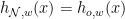. This computes a real-valued function, so where we’d like to use it for classification, we do so by thresholding, and abuse the notation to mean .

Some intuition for this definition would come from verifying that:

• Any function can be computed by a network of depth two and hidden neurons.
• The parity function can be computed by a network of depth two and hidden neurons. (NB: this one is a bit more challenging.)

In practice, the network architecture (this DAG) is designed based on some domain knowledge, and its design can impact the predictor that’s later selected by SGD. One default architecture, useful in the absence of domain knowledge, is the multi-layer perceptron, comprised of layers of complete bipartite graphs:

Convolutional nets capture the notion of spatial input locality in signals such as images and audio.⁴ In the toy example drawn, each clustered triple of neurons is a so-called convolution filter applied to two components below it. In image domains, convolutions filters are two-dimensional and capture responses to spatial 2-D patches of the image or of an intermediate layer.

Training a neural net comprises (i) initialization, and (ii) iterative optimization run until for sufficiently many examples . The initialization step sets the starting values of the weights at random:

(Glorot initialization.) Draw weights from centered Gaussians with variance and biases from independent standard Gaussians.⁵

While other initialization schemes exists, this one is canonical, simple, and, as the reader can verify, satisfies for every neuron and input .

The optimization step is essentially a local search method from the initial point, using stochastic gradient descent (SGD) or a variant thereof.⁶ To apply SGD, we need a function suitable for descent, and we’ll use the commonplace logistic loss , which bounds the zero-one loss from above:

 

Define . Note that , so finding weights for which the upper bound is small enough implies low error in turn. Meanwhile, is amenable to iterative gradient-based minimization.

Given samples from , stochastic gradient descent creates an unbiased estimate of the gradient at each step by drawing a batch of i.i.d. samples from . The gradient at a point can be computed efficiently by the backpropagation algorithm.

In more complete detail, our prototypical neural network training algorithm is as follows. On input a network , an iteration count , a batch size , and a step size :

Algorithm: SGDNN

1. Let be random weights sampled per Glorot initialization
2. For :
   1. Sample a batch , where are i.i.d. samples from .
   2. Update , where.
3. Output

PAC learning

Learning a predictor from example data is a general task, and a hard one in the worst case. We cannot efficiently (i.e. in time) compute, let alone learn, general functions from to . In fact, any learning algorithm that is guaranteed to succeed in general (i.e. with any target predictor over any data distribution ) runs, in the worst case, in time exponential in . This is true even for rather weak definitions of “success,” such as finding a predictor with error less than , i.e. one that slightly outperforms a random guess.

While it is impossible to efficiently learn general functions under general distributions, it might still be possible to learn efficiently under some assumptions on the target or the distribution . Charting out such assumptions is the realm of learning theorists: by now, they’ve built up a broad catalog of function classes, and have studied the complexity of learning when the target function is in each such class. Although their primary aim has been to develop theory, the potential guidance for practice is easy to imagine: if one’s application domain happens to be modeled well by one of these easily-learnable function classes, there’s a corresponding learning algorithm to consider as well.

The vanilla PAC model makes no assumptions on the data distribution , but it does assume the target belongs to some simple, predefined class . Formally, a PAC learning problem is defined by a function class⁷ . A learning algorithm learns the class if, whenever , and provided , it runs in time , and returns a function of error at most , with probability at least 0.9. Note that:

1. The learning algorithm need not return a function from the learnt class.
2. The polynomial-time requirement means in particular that the learning algorithm cannot output a complete truth table, as its size would be exponential. Instead, it must output a short description of a hypothesis that can be evaluated in polynomial time.

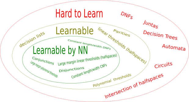
For a taste of the computational learning theory literature, here are some of the function classes studied by theorists over the years:

1. Linear thresholds (halfspaces): functions that map a halfspace to 1 and its complement to -1. Formally, functions of the form for some , where when and when .
2. Large-margin linear thresholds: forthe class
3. Intersections of halfspaces: functions that map an intersection of polynomially many halfspaces to and its complement to .
4. Polynomial threshold functions: thresholds of constant-degree polynomials.
5. Large-margin polynomial threshold functions: the class

1. Decision trees, deterministic automata, and DNF formulas of polynomial size.
2. Monotone conjunctions: functions that, for some map to if for all , and to otherwise.
3. Parities: functions of the form for some .
4. Juntas: functions that depend on at most variables.

Learning theorists look at these function classes and work to distinguish those that are efficiently learnable from those that are hard to learn. They establish hardness results by reduction from other computational problems that are conjectured to be hard, such as random XOR-SAT (though none today are conditioned outright on NP hardness); see for example these two results. Meanwhile, halfspaces are learnable by linear programming. Parities, or more generally, -linear functions for a field , are learnable by Gaussian elimination. In turn, via reductions, many other classes are efficiently learnable. This includes polynomial thresholds, decision lists, and more. To give an idea of what’s known in the literature, here is an artist’s depiction of some of what’s currently known:

 

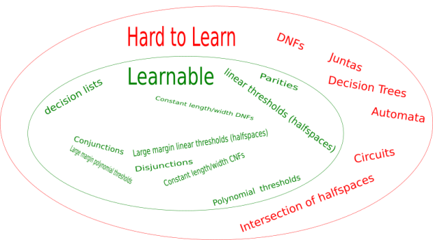
At a high-level, the upshot from all of this—and if you take away just one thing from this quick tour of PAC—is that:

Barring a small handful of exceptions, all known efficiently learnable classes can be reduced to halfspaces or -linear functions.

Or, to put it more bluntly, the state of the art in PAC-learnability is essentially linear prediction.

PAC analyzing neural nets

Research in algorithms and complexity often follows these steps:

1. define a computational problem,
2. design an algorithm that solves it, and then
3. establish bounds on the resource requirements of that algorithm.

A bound on the algorithm’s performance forms, in turn, a bound on the computational problem’s inherent complexity.

By contrast, we have already decided on our SGDNN algorithm, and we’d like to attain some grasp on its capabilities. So we’d like to do things in a different order:

1. define an algorithm (done),
2. design a computational problem to which the algorithm can be applied, and then
3. establish bounds on the resource requirements of the algorithm in solving the problem.

Our computational problem will be a PAC learning problem, corresponding to a function class. For SGDNN, an ambitious function class we might consider is the class of all functions realizable by the network. But if we were to follow this approach, we would run up against the same hardness results mentioned before.

So instead, we’ve established the theorem stated at the top of this post. That is, that SGDNN, over a range of network configurations, learns a class that we already know to be learnable: large margin polynomial thresholds. Restated:

Theorem, again: There is a choice of SGDNN step size and number of steps , as well as a with parameter , where , such that SGDNN on a multi-layer perceptron of depth between 2 and , and of width⁸ , learns large magin polynomials.

How rich are large margin polynomials? They contain disjunctions, conjunctions, DNF and CNF formulas with a constant many terms, DNF and CNF formulas with a constant many literals in each term. By corollary, SGDNN can PAC learn these classes as well. And at this point, we’ve covered a considerable fraction of the function classes known to be poly-time PAC learnable by any method.

Exceptions include constant-degree polynomial thresholds with no restriction on the coefficients, decision lists, and parities. It is well known that SGDNN cannot learn parities, and in ongoing work with Vitaly Feldman, we show that SGDNN cannot learn decision lists nor constant-degree polynomial thresholds with unrestricted coefficients. So the picture becomes more clear:

 

The theorem above runs SGDNN with a multi-layer perceptron. What happens if we change the network architecture? It can be shown then that SGDNN learns a qualitatively different function class. For instance, with convolutional networks, the learnable functions include certain polynomials of super-constant degree.

A word on the proof

The path to the theorem traverses two papers. There’s a corresponding outline for the proof.

The first step is to show that, with high probability, the Glorot random initialization renders the network in a state where the final hidden layer (just before the output node) is rich enough to approximate all large-margin polynomial threshold functions (LMPTs). Namely, every LMPT can be approximated by the network up to some setting of the weights that enter the output neuron (all remaining weights random). The tools for this part of the proof include (i) the connection between kernels and random features, (ii) a characterization of symmetric kernels of the sphere, and (iii) a variety of properties of Hermite polynomials. It’s described in our 2016 paper.

An upshot of this correspondence is that if we run SGD only on the top layer of a network, leaving the remaining weights as they were randomly initialized, we learn LMPTs. (Remember when we said that we won’t beat what a linear predictor can do? There it is again.) The second step of the proof, then, is to show that the correspondence continues to hold even if we train all the weights. In the assumed setting (e.g. provided at most logarithmic depth, sufficient width, and so forth), what’s represented in the final hidden layer changes sufficiently slowly that, over the course of SGDNN’s iterations, it remains rich enough to approximate all LMPTs. The final layer does the remaining work of picking out the right LMPT. The argument is in Amit’s 2017 paper.

PACing up

To what extent should we be satisfied, knowing that our algorithm of interest (SGDNN) can solve a (computationally) easy problem?

On the positive side, we’ve managed to say something at all about neural network training in the PAC framework. Roughly speaking, some class of non-trivially layered neural networks, trained as they typically are, learns any known learnable function class that isn’t “too sensitive.” It’s also appealing that the function classes vary across different architectures.

On the pessimistic side, we’re confronted to a major limitation on the “function class” perspective, prevalent in PAC analysis and elsewhere in learning theory. All of the classes that SGDNN learns, under the assumptions touched on in this post, are so-called large-margin classes. Large-margin classes are essentially linear predictors over a fixed and data-independent embedding of input examples, as alluded to before. These are inherently “shallow models.”

That seems rather problematic in pursuing any kind of theory for learning layered networks, where the entire working premise is that a deep network uses its hidden layers to learn a representation adapted to the example domain. Our analysis—both its goal and its proof—clash with this intuition: it works out that a “shallow model” can be learned when assumptions imply that “not too much” change takes place in hidden layers. It seems that the representation learning phenomenon is what’s interesting, yet the typical PAC approach, as well as the analysis touched on in this post, all avoid capturing it.

---

1. Here is the dimension of the instance space.↩
2. For instance, ReLU activations, of the form .↩
3. Recurrent networks allow for cycles, but in this post we stick to DAGs.↩
4. Convolutional networks often also constrain subsets of their weights to be equal; that turns out not to bear much on this post.↩
5. Although not essential to the results described, it also simplifies this post to zero the weights on edges incident to the output node as part of the initialization.↩
6. Variants of SGD are used in practice, including algorithms used elsewhere in optimization (e.g. SGD with momentum, AdaGrad) or techniques developed more specifically for neural nets (e.g. RMSprop, Adam, batch norm). We’ll stick to plain SGD.↩
7. More accurately, a sequence of function classes for .↩
8. The width of a multi-layer perceptron is the number of neurons in each hidden layer.↩