
Backpropagation ≠ Chain Rule

The chain rule is a fundamental result in calculus. Roughly speaking, it states that if a variable 


Besides being a handy tool for computing derivatives in calculus homework, the chain rule is closely related to the backpropagation algorithm that is widely-used for computing derivatives (gradients) in neural network training. This blog post by Boaz Barak is a beautiful tutorial on the chain rule and the backpropagation algorithm.
As in Barak’s post, the backpropagation algorithm is usually taught as an application of the chain rule in machine learning classes. This leads to a common belief that “backpropagation is just applying the chain rule repeatedly”. While this is in a sense true, we wish to point out in this blog post that this belief is over-simplifying and can lead to incorrect implementations of the backpropagation algorithm. It has been discussed in many blog posts that backpropagation is not just the chain rule, but we want to focus on a simple and basic difference here.

Consider the “neural network” above: it consists of an input variable 


Using the chain rule (1) twice, we can compute the derivative

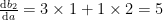
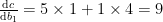
Backpropagation computes the derivative

In the calculations above, note the difference between partial and full derivatives. For example, the partial derivative 

Now it should be clear that equation (3) cannot be directly explained as the standard chain rule (1). The key difference is that in the chain rule, we need partial derivatives of a single variable w.r.t. multiple other variables, whereas in (3), we need partial derivatives of multiple variables w.r.t. the same variable.
Of course, one can prove the correctness of backpropagation using the chain rule in various ways, but the simple proof “backpropagation uses the standard chain rule at every step” is incomplete. Also, it is certainly possible to compute derivatives (gradients) on a neural network directly using the chain rule similarly to (2), but in neural network training one typically wants to calculate the derivatives of a single output variable w.r.t. a large number of input variables, in which case backpropagation allows a more efficient implementation than using the standard chain rule directly.
The real chain rule in actual backpropagation
When implementing the backpropagation algorithm, it is more convenient and efficient to add in the two terms (or any number of terms in general) on the right-hand-side of (3) at different steps of the algorithm. This is described in Barak’s tutorial, which also has an actual Python implementation! In contrast to the failure of naively explaining equation (3) as the chain rule, there is a way to explain this implementation using the chain rule directly.
To describe the implementation, suppose 


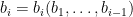

For each variable 


Of course, it suffices to update 
The update rule (4) can be explained as a direct application of the chain rule as follows. If we know the values of 


By the chain rule,
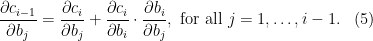
The correspondence between (4) and (5) completes the explanation: if 


Thanks! I think in theory terms, the way to describe it is as follows: if you follow the chain rule in the standard “forward” direction as we learned in basic calculus, you will pay a price that scales in the *formula size* for the output.
Backpropagation allows us to pay a price that only scales with the *circuit size*. This is what enables automatic differentiation since a computation graph is simply a circuit.
I still maintain that it’s the (multivariate) chain rule, but it applied in a clever way.
LikeLiked by 1 person
Thanks for the reply! Just to make a small clarification: if a circuit has only one input variable, there is a way to implement the “forward chain rule” algorithm efficiently (with “time” complexity proportional to the circuit size) via dynamic programming, no matter how many output variables we have. When there are m input variables, doing this for each input variable achieves complexity roughly m * circuit size, which can be much smaller than the formula size. By operating in the reversed direction, backpropagation replaces m by the number of *output* variables. This is a significant improvement because there is usually only one output variable but a huge number m of input variables. To achieve this, backpropagation applies a reversed version of the chain rule like in (3). The difference between the reversed version and the standard version is usually neglected, partly because they are the “same thing” if, for example, there is no edge from b_1 to b_2 in the example. Adding the edge highlights the difference.
One purpose of this blog post is to show that backpropogation is an arguably non-trivial algorithm, despite its simplicity (which is a lesson that I failed to learn when I was an undergrad…) Thank you for your contribution in helping more people appreciate the ideas behind the backpropagation algorithm!
LikeLike
Thank you! That’s a good point. Note also that m * circuit_size complexity can be achieved via numerical differentiation
LikeLiked by 1 person